Sales Price Variance

Definition

Sales Price Variance is the measure of change in sales revenue as a result of variance between actual and standard selling price.

Formula

Sales Price Variance:

=	(Actual Price - Standard Price)	x	Actual Unit
=	Actual Price x Actual Units Sold	-	Standard Price x Actual Units Sold
=	Actual Sales Revenue	-	Standard Revenue of Actual Units Sold

Explanation

Sales Price Variance can be calculated in a number of ways as illustrated in the formulas given above. The calculation of the variance is in fact very simple if you just remember the objective of finding the variance, i.e. how much change in sales revenue is attributable to the change in selling price from the standard?

Example

ABC PLC is a fertilizer producer which specializes in the manufacture of NHK-II (a chemical fertilizer) and ORG-I (a types of organic fertilizer).

Following information relates to the sale of fertilizers by ABC PLC during the period:

Material	Quantity	Acutal Price	Standard Price
NHK-II	200 tons	Rs.380/ton	Rs.400/ton
ORG-I	300 tons	Rs.660/ton	Rs.600/ton

---

Sales Price Variance shall be calculated as follows:

	Actual Price (a)	Standard Price (b)	a - b = c	Unit Sold (d) (tons)	c x d
NHK-II	380	400	20	200	4,000 Adverse
ORG-I	660	600	60	300	18,000 Favorable
Total					14,000 Favorable

Analysis

Favorable sales price variance suggests higher selling price realized during the period than anticipated in the standard. Reasons for favorable sales price variance may include:

• Decrease in the number of competitors in the market
• Improved product differentiation and market segmentation
• Better promotion and aggressive sales campaign

Adverse sales price variance indicates that sales were made at a lower average price than the standard. Causes for adverse sales price variance may include:

• Increase in competition in the market
• Decrease in demand for the products
• Reduction in price enforced by regulatory authorities.

The Cambridge Version of the Quan­tity Theory

Explanation to the Theory:

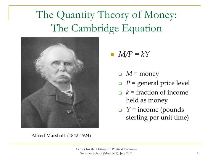
The Cambridge economists—like Alfred Marshall and A. C. Pigou—presented an alter­native to Fisher’s version of Quantity Theory.

They have attempted to establish that the Quantity Theory of Money is a theory of demand for money (or liquidity preference). The Cambridge version of the Quantity Theory of Money is now presented.

Formally, the Cambridge equation is identical with the income version of Fisher’s equation: M = kPY, where k = 1/V in the Fisher’s equation.

Here 1/V = M/PT measures the amount of money required per unit of transactions and its inverse V measures the rate of turnover or each unit of money per period.

So if k and Y remain constant, P is directly proportional to the initial quantity of money (M).

Criticisms:

1. The Chain of Causation:

Critics argued that all the factors in the equation of exchange are variables and statistical studies have shown that they are interrelated. Moreover, the line of causation is not always from M (money supply) to P (the price level). It may be from V to P. A change in the rate of spending, all the other factors remaining the same, will result in a change in prices just as surely as would a change in the Quantity Theory of money, other things remaining the same.

Or a change in T, other things remaining the same, will cause a change in prices. So it is difficult to accept the theory that changes in the quantity of money are always the causes in the price level. Studies have shown that the price level cannot be easily and quickly controlled by changing the amount of money and credit available for the purchase of goods and services.

It may also be said that, under certain circumstances, an increase in the quantity of money will not produce any change in the price level. Keynes has pointed out that the Quantity Theory is inapplicable to a country which has unemployed resources (capital and labour not in use).

In such a country, creation of more money will lead to more employment and higher production (larger supply of goods) and no change in the price level. Prices will change in proportion to money supply only when there is no scope for increasing production, i.e., when there are no unemployed resources in the economy.

2. There are Inactive Balances:

Under Fisher’s formula, the price level depends upon the total quantity of money. But it is only a part of the total quantity of money which influences prices. There always exist inactive balances (hoards) which exert no pressure at all on the prices of goods and services. This is clearly seen during depressions.

3. Simultaneous Changes:

The Quantity liquation cannot be used for analysing the effects, of changes in M, or T, on the price level except on the ceteris paribus assumption, “other things remaining constant.” But in the case of monetary variables such an assumption cannot be made. When M changes, T and V both change. When T changes, M, and V change. The net effect on the price level of a change in any of the variables of the quantity equation depends on how the other variables are simultaneously changed.

4. The Process of Change:

Theory does not show the process through which changes in the amount of money affect the price level. Keynes put great emphasis on this point.

He observed that:

“The fundamental problem of monetary theory is not merely to establish identities or statistical relation but to treat the problem dynamically, analysing the different ele­ments involved in such a manner as to exhibit the causal processes by which the price-level is determined and the method of transition from one equilibrium to another.”

5. The Assumption of Full Employment:

ADVERTISEMENTS:

So increase in the quantity of money does not always increase prices. If there are unem­ployed resources, increase of money increases employment and not prices. As Keynes points out, the Quantity Theory is based on the assumption of Full Employment.

6. The Value of Money Determines the Quan­tity of Money:

According to Quantity Theory, an increase in the supply of goods or it will cause a fall in the price level P. Monetary and banking practices, increases in the supply of goods always leads to an increase in the supply of money (through creation of credit and otherwise). M therefore, depends on T; they are not independent variables. If this view is correct, the value of money is not deter­mined by its quantity; on the contrary it is the value of money which determines its quan­tity.

7. Non-Monetary Factors:

Prices may change and the value of money vary for reasons entirely unconnected with the quantity of money.

Some examples are given below:

(i) Changes in the level of efficiency wages may change costs of production and affect prices.

(ii) If increase of output occurs under con­ditions of diminishing returns, marginal costs will rise and prices will rise. Similarly, prices will fall if production increases under con­ditions of increasing returns.

(iii) Increase and decrease of monopoly power will, respectively, increase and decrease prices.

(iv) Prices are affected by variations in effective demand or expenditure. Consumption expenditure and investment expenditure both vary—as also the proportion between them.

8. Misleading Emphasis:

Finally, according to Crowther the Quantity Theory puts a mis­leading emphasis on the importance of the quantity of money as the cause of price changes and pays too much attention on the level of prices. In the short rim these principles of the Quantity Theory are not in accord with facts. In actual life the price level and volume of production move up and down in a cyclical pattern.

The Quantity Theory draws pointed attention to one important factor which causes price change, viz., the quantity of money. It is admitted that the quantity formula “hides many links in the chain of causation”, but it is undisputed that the formula gives us a rough and ready method of determining the effects of changes in the quantity of money and certain other factors influencing the price level.

From the above discussion it is clear that the Quantity Theory is inadequate and defec­tive. It has, however, certain merits. Generally, we find that when money supply increases, the price level rises. For example, during 1939-45 in India there was a large increase in the volume of notes and bank advances and the price level rose very fast. Hence, there is some relationship between the quantity of money and the value of money. The Quantity Theory states the relationship not with absolute correctness but only approximately.

Dr. Milton Friedman (the 1976 Nobel Prize winner) believes that the quantity theory of money is true in its simple or cured form, i.e., price (P) varies with quantity of money (M). He believes that there is a proportionality between the quantity of money and the general price level in an economy.

Purchasing power parity

When making comparisons between countries which use different currencies it is necessary to convert values, such as national income (GDP), to a common currency.

This can be done it two ways:

1.   Using market exchanges rates, such as $1 = ¥200, or:

2.   Using purchasing power parities (PPPs)

Market exchange rates

Using market exchange rates creates two main difficulties:

Firstly, market exchange rates can quickly change, which artificially changes the value of the variable in question, such as GDP. For example, a one-month appreciation of the US$ by 5% against the Japanese Yen would reduce the dollar value of the Japanese economy by 5%. Clearly, this is more to do with changes in the exchange rate than changes in the underlying state of the Japanese economy.

Secondly, market exchange rates are determined by demand and supply of currencies, which reflect changes in imports and exports of traded goods and services. However, not all countries trade the same proportion of their income and output, so currency values are not determined on a consistent basis.

Purchasing power parity

The alternative to using market exchange rates is to use purchasing power parities (PPPs). The purchasing power of a currency refers to the quantity of the currency needed to purchase a given unit of a good, or common basket of goods and services. Purchasing power is clearly determined by the relative cost of living and inflation rates in different countries. Purchasing power parity means equalising the purchasing power of two currencies by taking into account these cost of living and inflation differences.

For example, if we convert GDP in Japan to US dollars using market exchange rates, relative purchasing power is not taken into account, and the validity of the comparison is weakened. By adjusting rates to take into account local purchasing power differences, known as PPP adjusted exchange rates, international comparisons are more valid.

Materiality Concept in Accounting

The materiality concept helps ensure that firms do not withhold critical information from investors, owners, lenders, and regulators.

What is the Materiality Concept?

The materiality concept is the principle in accounting and financial accounting and reporting that firms may disregard trivial matters, but they must disclose everything that is important to the report audience. Items that are important enough to matter are material items.

United States GAAP, for instance, states that items are material if "they could ... influence the economic decisions of [financial statement] users…". In other words, materiality errors can mislead decision makers.

Note that the materiality concept has meaning for any financial statement only concerning:

• The statement's intended audience.
• The statement's purpose for this audience.

When an independent auditor reviews a firm's financial statements, the best possible outcome is an auditor's opinion of Unqualified. This opinion affirms the auditor's judgment that the reports are accurate and conform to GAAP. And, this means the auditor finds no materiality issues.

Materiality Depends On the Purpose and the Audience

The first answer to that question is the following: "Materiality depends on the purpose of the financial report and its intended audience."

Consider, for instance, a firm's financial reports for the period just ended. Different versions of the statements can serve different audiences for different purposes.

Financial Statement Audience 1
Materiality in the Annual Report to Shareholders

The Annual Report to shareholders includes one version of the firm's statements. Here, the firm is legally responsible for publishing statements that serve two purposes.

• Firstly, statements must enable shareholders to make informed decisions when electing directors. The firm, therefore, must disclose information about individual candidates that could influence a voting decision. Information for this purpose could include, for instance, information about potential conflicts of interest or family ties with the firm's officers.
• Secondly, these statements enable shareholders and investors to evaluate the firm's recent financial results and prospects for future business. As a result, the materiality concept requires full disclosure on everything that could influence a decision to hold, buy, or sell shares of stock. Relevant information here could include, for example::
• Transparent interpretation of recent performance
  For this purpose, firms sometimes supplement GAAP-required metrics such as Net Income with particular income metrics such as EBITDA (Earnings before interest, taxes, depreciation, and Amortization)
• Analysis of the firm's competitive situation
• Disclosure of forthcoming lawsuits or government penalties

Financial Statement Audience 2
Materiality For Lenders and Bond Rating Agencies

Potential lenders and bond rating agencies are another report audience. This audience, of course, must judge the firm's creditworthiness. Here, the audience tries to answer questions such as these:

• Firstly, can the company service it's debt load if it takes on still more debt?
• Secondly, what is the firm's level of leverage?
• Thirdly, what are the firm's earnings prospects in its core line of business?

The audience must have enough detail to address such questions seriously. Here, the audience needs full disclosure on the firm's creditors, liabilities, and investments. They also need full disclosure on planned changes to the firm's business model and strategies. And, they must know which financial and business risks the firm faces.

Financial Statement Audience 3
Materiality For Potential Mergers and Acquisitions

Here, each potential partner must know the other business accurately and in detail. Each must know, in other words, the other party's:

• Business model. The business model reveals, for instance, which of the firm's products earn healthy margins and which do not.
• Cost structure. This structure describes the kinds and relative proportions of fixed and variable costs that a firm incurs.
• Capital and financial structures. These structures define the firm's level of leverage. The structures show how the firm's creditors and owners share business risks and rewards.
• Organization and governance structures.
• Marketing strategy and selling model.

All potential partners need this information, in advance. Everyone must know what each adds to partnership production, marketing, selling, and general management. And, they must plan together how to eliminate redundancies and overly costly operations. And, each must know the risks and liabilities that the others bring to the partnership. Only with full knowledge in these areas can they make an informed decision on going forward joining together.

What Constitutes Materiality Abuse?

Abuses of the materiality concept in accounting can have serious legal consequences. Nevertheless, GAAP and FASB have resisted stating precisely an error size that qualifies as materiality abuse. In reviewing specific cases, however, auditors and courts use several "rules of thumb."

• On the Income statement, errors of 5% or more of before-tax Profit, or 0.5% of sales revenues, are more likely seen as "large enough to matter."
• On a Balance sheet, a questionable entry more than 0.3 to 0.5% of total assets, or more than 1% of total equity, is likely to be viewed suspiciously.

Abuse of the Materiality Concept

Those judging materiality must also consider other factors besides error magnitude. This requirement is no doubt one reason that regulators resist setting size criteria for materiality abuse. They also take into account two other factors:

• Firstly, Motivation and Intent Behind the Error.
   
  An abuse judgment is more likely if auditors or a court can prove intent to do any of the following:
  • Keep stock prices artificially high. 
  • Inflate reported earnings.
  • Understate the actual value of the asset base.
  • Inappropriately influence merger or acquisition decisions.
• Secondly, the Likely Effect on User Perceptions and Judgment.
  
  Consider for instance an Income statement placement error. Suppose there are significant "Manufacturing indirect labor expenses" for this period. Suppose also these are wrongly placed under "Direct manufacturing labor." That error probably does not qualify as materiality abuse. Regarding materiality, it is likely a harmless error because both kinds of expense contribute to cost of goods sold (COGS). As a result, the critical information for decision-makers—gross profits—is the same regardless of which COGS category has the indirect labor expense.
  
  However, suppose instead that the same indirect labor expenses appear wrongly below the gross profit line instead of above it. This kind of mistake may qualify as fraud. This mistake is harmful because the misstatement does inappropriately improve gross profits.

Substitution Effect...Micro Economics

Substitution Effect on the Changes in Consumption of a Good (with diagram)

The important factor responsible for the changes in consumption of a good is the substitution effect.

Whereas the income effect shows the change in the quantity purchased of a good by a consumer as a result of change in his income, prices of goods remaining constant, substitution effect means the change in the quantity purchased of a good as a consequence of a change in its relative price alone, real income or level of satisfaction remaining constant.

When the price of a good changes, he goes to a different indifference curve and his level of satisfaction changes. The Consumer goes to a different indifference curve as a result of a change in price because with this the real income or purchasing power of a consumer also changes. To keep the real income of the consumer constant so that the effect due to a change in the relative price alone may be known, price change is compensated by a simultaneous change in income.

For example, when price of a good, say X, falls, real income of the consumer would increase and he would be in equilibrium at a higher indifference curve showing a higher level of satisfaction. In order to find out the substitution effect i.e., change in the quantity of X purchased which has come about due to the change only in its relative price, the consumer’s money income must be reduced by an amount that cancels out the gain in real income that results from the decrease in price.

Now, two slightly different concepts of substitution effect have been developed; one by J.R. Hicks and the other by E. Slutsky. These two concepts of substitution effect have been named after their authors. Thus, the substitution effect which is propounded by Hicks and Allen is called the Hicksian Substitution Effect and that developed by E. Slutsky is known as Slutsky Substitution Effect. The two concepts differ in regard to the magnitude of the change in money income which should be effected so as to neutralise the change in real income of the consumer which results from a change in the price.We shall explain here the Hicksian substitution effect.

In the Hicksian substitution effect price change is accompanied by a so much change in money income that the consumer is neither better off nor worse off than before, that is, he is brought to the original level of satisfaction. In other words, money income of the consumer is changed by an amount which keeps the consumer on the same indifference curve on which he was before the change in the price.

Thus the Hicksian substitution effect takes place on the same indifference curve. The amount by which the money income of the consumer is changed so that the consumer is neither better off nor worse off than before is called compensating variation in income. In other words, compensating variation in income is a change in the income of the consumer which is just sufficient to compensate the consumer for a change in the price of a good.

Thus, in the Hicksian type of substitution effect, income is changed by the magnitude of the compensating variation in income. Hicksian substitution effect is illustrated in Fig. 8.37. With a given money income and given prices of the two goods as represented by the budget line PL, the consumer is in equilibrium at point Q on the indifference curve IC and is purchasing OM of good X and ON of good Y.

Suppose that the price of good X falls (price of Y remaining unchan­ged) so that the budget line now shifts to PL’. With the fall in price of X the consumer’s real income or purchasing power would increase. In order to find out the substitution effect, this gain in real income should be wiped out by reducing the money income of the consumer by such an amount that forces him to remain on the same indifference curve IC on which he was before the change in price of the good X.

When some money is taken away from the consumer to cancel out the gain in real income, then the budget line which shifted to position PL’ will now shift downward but will be parallel to PL’. In Fig.8.37 a budget line AB parallel to PL’ has been drawn at such a distance from PL’ that it touches the indifference curve IC.

It means that reduction of consumer’s income by the amount PA (in terms of Y) or L’B (in terms of X) has been made so as to keep him on the same indifference curve. PA or L’B is thus just sufficient to cancel out the gain in the real income which occurred due to the fall in the price of X. PA or L’B is therefore compensating variation in income.

Now, budget line AB represents the new relative prices of goods X and Y since it is parallel to the budget line PL’ which was obtained when price of good X and fallen. In comparison to the budget line PL, X is now relatively cheaper. The consumer would therefore rearrange his purchases of X and Y and will substitute X for Y.

That is, since X is now relatively cheaper and Vis now relatively dearer than before, he will buy more of X and less of Y It will be seen from Fig. 8.37 that budget line AB represents the changed relative prices but a lower money income than that of PL, since consumer’s income has been reduced by compensating variation in income.

It will seen from Fig. 8.37 that with budget line AB the consumer is in equilibrium at point Y and is now buying OM’ of X and ON’ of Y. Thus in order to buy X more he moves on the same indifference curve IC from point Q to point T. This increase in the quantity purchased of good X by MM’ and the decrease in the quantity purchased of good Y by NN’ is due to the change only in the relative prices of goods X and Y, since effect due to the gain in real income has been wiped out by making a simultaneous reduction in consumer’s income.

Therefore, movement from Q to T represents the substitution effect. Substitution effect on good X is the increase in its quantity purchased by MM and substitution effect on Y is the fall in its quantity purchased by MNT. It is thus clear that as a result of the Hicksian substitution effect the consumer remains on the same indifference curve; he is however in equilibrium at a different point from that at which he was before the change in price of good X.

The less the convexity of the indifference curve, the greater will be the substitution effect. As is known, the convexity of indifference curve is less in the case of those goods which are good substitutes. It is thus clear that the substitution effect in case of good substitutes will be large.

It is thus clear that a fall in relative price of a commodity always leads to the increase in its quantity demanded due to the substitution effect, the consumer’s satisfaction or indifference curve remaining the same. Thus the substitution effect is always negative.

The negative substitution effect implies that the relative price of a commodity and its quantity demanded change in opposite direction, that is, the decline in relative price of a commodity always causes increase in its quantity demanded. It is this negative substitution effect which lies at the root of the famous law of demand stating inverse relationship between price and quantity demanded.